Quick Context: f(x,y) = 0.5x^2 + 0.5*y^2 a constraint S: g(x,y) = 0.5x^2 + y^2 = 1 (ellipse) as the constraint is closed and bounded, f S must attain ... This video introduces a really intuitive way to solve a constrained optimization problem using
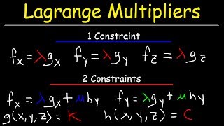
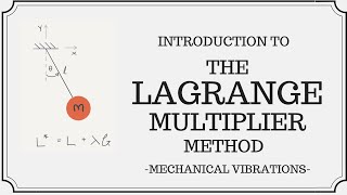
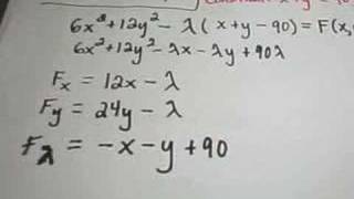
Visualization Of The Lagrange Multiplier Method -
f(x,y) = 0.5x^2 + 0.5*y^2 a constraint S: g(x,y) = 0.5x^2 + y^2 = 1 (ellipse) as the constraint is closed and bounded, f S must attain ... This video introduces a really intuitive way to solve a constrained optimization problem using
Important details found
- f(x,y) = 0.5x^2 + 0.5*y^2 a constraint S: g(x,y) = 0.5x^2 + y^2 = 1 (ellipse) as the constraint is closed and bounded, f S must attain ...
- This video introduces a really intuitive way to solve a constrained optimization problem using
Why this topic is useful
The goal of this page is to make Visualization Of The Lagrange Multiplier Method easier to scan, compare, and understand before opening related resources.
Sponsored
Frequently Asked Questions
What should readers check next?
Readers should check related pages, official references, or updated sources when details matter.
Why are related topics included?
Related topics help readers compare nearby references and understand the broader subject.
What is this page about?
This page summarizes Visualization Of The Lagrange Multiplier Method and connects it with related entries, references, and supporting context.
Supporting Images







Sponsored